Geometry of Basins of Attraction and Heteroclinic Connections in Coupled Bistable Systems
	Daniel Lyons, Joseph M. Mahaffy, Sara Wang, Antonio Palacios and Visarath In

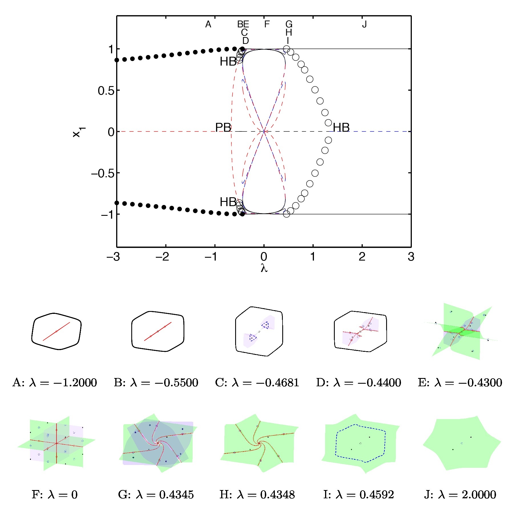
The image above provides a summary of the changes in the basins of attraction for our coupled bistable system given by the equation:

Movie

We have created a movie to view the changing basins of attraction as the coupling strength varies. Hyperlink to the movie.

Figures

Each of the figures were generated in MatLab. The paper only has eps figures showing a single perspective. However, the MatLab figures are 3D and can be rotated to any perspective desired. Below we show the figures from the paper and provide hyperlinks to the MatLab fig files, which when loaded into MatLab can be displayed and rotated to any desired viewing angle.

Programs

The paper "Geometry of Basins of Attraction and Heteroclinic Connections in Coupled Bistable Systems" has two appendices about the generation of the figures for the basins of attraction. Appendix A provides information about the numerical techniques employed to find equilibria and generate the stable manifolds or separatrices. Appendix B provides details about running the MatLab code for the generation of the figures seen above. For convenience, there is a hyperlink to acquire all the programs necessary to create the figures.

Hyperlink of CCFM_manifolds.zip

When CCFM_manfolds.zip is expanded, there are two Getting Started files and five folders containing the important files needed to generate the figures. We have divided the programs into the ones needed to generate Figures 2-12 and the files for the equilibria in Figure 13. The Getting Started files provide the necessary details to generate the figures with the equilibria and surfaces separating the basins of attraction. For additional information, the reader should read Appendix B from the paper.

Getting Started Stable Manifolds

To generate Figures 02-12 from the paper "Geometry of Basins of Attraction and Heteroclinic Connections in Coupled Bistable Systems" by Lyons et. al., follow these instructions:

(1) Start up MatLab and set the current directory to the "driver" folder.

(2) There are seven MatLab m-files in this folder. Each of these m-files may be used to generate one or multiple figures from the paper. If you want to reproduce a particular figure from the paper, refer to Appendix B in the paper to determine which particular driver file to use. Once you have selected a driver file, open this file in MatLab.

(3) Each MatLab driver m-file calls multiple MatLab functions from the folder "functions". In order to run any of the driver files, it is important for MatLab to be able to locate this folder. To do this, a line near the beginning of the driver file must be modified once so that it can find the directory that has "/CCFM_manifolds/functions/" inside. To do this, find the
string variable called "mypath" near the beginning of the file and change it to the current filepath leading up to the "CCFM_manifolds" directory. For example, if you are using the driver file "manifold_1D_stable.m", and your filepath structure is"/Users/myname/small_folder/CCFM_manifolds/functions/", then you should go to line 11 and change the "mypath" string variable on line 11 to "/Users/myname/small_folder/". Note that the MatLab driver file will not run if you do not complete this step correctly.

(4) Run/execute the MatLab driver file. There will likely be some output printed out, but the program should run without error.

(5) Note that some of the MatLab driver programs work for multiple values of the bifurcation parameter lambda. Recall from the paper that changing lambda may lead to a change in the number and type of equilibria in the system. As a result, to generate the stable manifolds for a different lambda value than the default one in the code, it is necessary to change a few lines of code in the driver file. Refer to the appropriate section of Appendix B in the paper and carefully read and follow the corresponding instructions to do this. Also, some parameters may need to be changing in the driver file based on which lambda value is used. Refer to Appendix A to determine which parameters to change and the appropriate values.

Getting Started Equilibria

The instructions below may be followed to generate the plot of the 27 equilibria (Figure 13):

(1) Start up MatLab and set the current directory to the "equilibria" folder.

(2) Open the MatLab script "CCFM_equilibria_lambda_color.m".

(3) Run this MatLab script.

Acknowledgements
A.P. was supported by the Complex Dynamics and Systems Program of the Army Research Office, supervised by Dr. Samuel Stanton, under grant W911NF-07-R-003-4. A.P. was also supported by the ONR Summer Faculty Research Program, at SPAWAR Systems Center, San Diego. V.I. acknowledges support from the Office of Naval Research (Code 30) and the SPAWAR internal research funding (S\&T) program.